#| label: setup-packages
#| echo: false
#| message: false
#| warning: false
#| results: "hide"

packages <- c(
  "tidyverse", "knitr", "data.table", "DT", "here", "kableExtra",
  "lme4", "openxlsx", "readxl", "wesanderson", "stringr",
  "itsadug", "mgcv", "report", "gratia", "ggrepel", "gridExtra"
)

installed_packages <- rownames(installed.packages())
to_install <- setdiff(packages, installed_packages)

if (length(to_install) > 0) {
  suppressMessages(install.packages(to_install))
}


invisible(lapply(packages, function(pkg) {
  suppressMessages(suppressWarnings(library(pkg, character.only = TRUE)))
}))

#Set working directory where this Rmd file lives
setwd(here::here())

# Load data
  romall<-readxl::read_excel("romall_new_pub.xlsx")

nc<-readxl::read_excel("noncaus_new_pub.xlsx")Causalness, frequency, diachrony and the causal-noncausal alternation in Italian and Spanish
Corpus Linguistics and Linguistic Theory - final submission December 2025
Giulia Mazzola 
Guglielmo Inglese
![]()
Replication materials for: Mazzola & Inglese, “Causalness, frequency, diachrony and the causal-noncausal alternation in Italian and Spanish” in Corpus Linguistics and Linguistic Theory (Accepted December 2025). Full citation information will be released after publication.
Part I: Calculating the causalness degree over time
Cross-linguistic work on the causal-noncausal alternation has shown that there exists a strong correlation between the frequency of use of a given verb in causal vs. noncausal contexts and its preferred coding pattern for the alternation, with verbs typically occurring in causal contexts preferably selecting the anticausative pattern (Haspelmath et al. 2014). These findings rest upon the assumption that the correlation between frequency and coding is diachronic in nature, but this has so far not been tested on historical data.
Data for this study comes from diachronic corpora of Italian (MIDIA, D’Achille & Iacobini 2022) and Spanish (CDH, Real Academia Española 2013), from which the tokens of the 20 verb meanings used in Haspelmath et al. (2014) have been extracted and richly annotated. Each token has been classified according to whether it occurs in a causal or a noncausal context (following Haspelmath et al. 2014: 603, we considered passive, impersonal, reflexive, and reciprocal usages as causal) and based on the type of marking, that is, zero marking, marked anticausative (mainly with the reflexive marker si/se), or marked causative (regardless of the type of auxiliary verb, e.g., fare/hacer ‘make’, lasciare/dejar ‘let’, etc.).
Our dataset romall includes causal and noncausal observations. The subset nc only contains noncausal observations, and only includes “the variable contexts”, only verb lemma with alternation between zero and anticausative marking, since from a variationist point of view is important to only look at contexts where the variation actually occurs.
If we zoom in onto the panchronic percentage of noncausal usage of the verbs and plot them against the spontaneity scale (or causative prominence) proposed by Haspelmath (1993), we can observe that Italian and Spanish substantially behaves like other languages in the sample studied by Haspelmath et al. (2014). Although the data in the plot below displays the expected trend, the results may be problematic in that the percentage of noncausal usages has been calculated over the entire Italian and Spanish datasets. The problem is that, since the data comes from diachronic corpora, one cannot be sure of the accuracy of this measurement, as the causalness degree may in fact be variable over time.
## Script for Figure 2

result_noncaus_meaning <- romall %>%
  group_by(language, meaning) %>%
  summarise(noncaus = sum(semantics == 'noncaus') * 100 / n())

plot_noncaus_tot <- ggplot(result_noncaus_meaning, aes(x = meaning, y = noncaus, color = language, group = language)) +
  geom_smooth(aes(y = noncaus, color = language), method = 'loess', se = FALSE) +
  labs(y = "% noncausal usage", x = "Causative prominence") +
  scale_color_manual(
    values = c("italian" = "gray70", "spanish" = "gray20"),
    labels = c("italian" = "Italian", "spanish" = "Spanish")) +
  coord_cartesian(ylim = c(1, 100)) +
  theme_minimal() +
  theme(
    panel.grid.major = element_blank(),
    panel.grid.minor = element_blank(),
    panel.background = element_rect(fill = "white", color = NA),
    axis.text.x = element_text(angle = 90, vjust = 0.5, hjust=1)  # Rotate x-axis labels
  )

custom_order <- c("split", "close", "break", "open", "gather", "connect", "rock", "improve", "rise", "fill", "burn", "turn", "stop", "melt", "sink", "go out", "wake up", "dry", "boil")
plot_noncaus_tot <- plot_noncaus_tot + scale_x_discrete(limits = custom_order)
print(plot_noncaus_tot)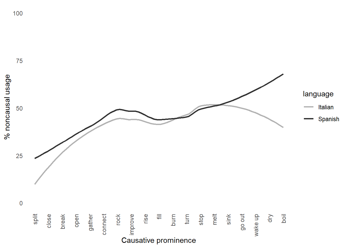
Overall purpose
We would like to include a new predictor in our dataset, namely the proportions of causal transitive uses (vs. non causal uses) of the verbs by time, which we define as causalness degree. In order to do so we need to come up with a periodisation for our data (spanning between 1140 and 2001), which allows to calculate the relative frequency of causal uses by time. To reach a periodisation, a visual survey of the data can be instructive, it might pose the problem of the analyst’s bias, as “different researchers may arrive at different groupings even for the same data set” (Gries & Hilpert 2008:2).
Variability neighbour clustering (VNC)
Gries & Hilpert (2008) propose a more accurate method to come up with meaningful periodisation for a given dataset: Variability-based Neighbor Clustering (VNC). It is similar to hierarchical cluster analysis (HCA), i.e. a method that displays a hierarchy of clusters, typically in the form of dendrograms with branches and leaves. Differently from HCA, VNC does justice to the chronological linearity of linguistic developments by not separating adjacent periods, and shows significant differences between periods based on the standard deviation, which is taken as similarity measure and averaging as amalgamation rule.
The analyst needs to input the proportions of a given variant (in our case, causal uses) for periods, ideally decades. The choice of the periods size is somewhat arbitrary, but making different attempts helps to find the right balance between data sparsity and significance of the VNC results. Because at various points in the diachrony of our dataset data are scarce (see Histogram), we started with periods of 20 years and ended up with periods of 70 years. The VNC periodisation based on periods of 70 years is the one with the best results in statistical terms, as the standard deviation measure for different periods are large enough to show significant differences. Hereby we show the procedure.
ggplot(romall, aes(x=year, fill=semantics)) +
  geom_histogram(alpha = 0.5, position="stack") +
  facet_wrap(~stringr::str_to_title(language))+
  scale_fill_manual(labels=c("Causal", "Noncausal"), values= (c("#fc8961", "#b73779")))+   theme_minimal()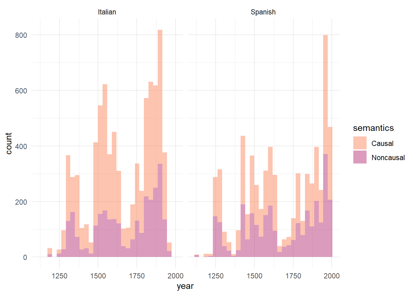
Establish the 70-years periodisation
- Step 1: Split the Italian and Spanish dataset.
# Step 1
esp <- filter(romall, language=="spanish")
ita <- filter(romall, language=="italian")
The range of years in the italian dataset is 1200, 1968 and for Spanish 1140, 2001.
- Step 2: Create a new variable with the years groups in 70-years periods. Periods are indicated with the central years in the 70 years span, i.e. 1175 stands for the period between 1140 and 1210.
# Step 2
esp<-esp %>%
  mutate(
    period70_es=case_when(
      year<1210 ~ "1175",
      year<1280 ~ "1245",
      year<1350 ~ "1315",
      year<1420 ~ "1385",
      year<1490 ~ "1455",
      year<1560 ~ "1525",
      year<1630 ~ "1595",
      year<1700 ~ "1665",
      year<1770 ~ "1735",
      year<1840 ~ "1805",
      year<1910 ~ "1875",
      year<1980 ~ "1945",
      year<=2001 ~ "1990"
    )
  )

ita<-ita %>%
  mutate(
    period70_ita=case_when(
      year<1270 ~ "1235",
      year<1340 ~ "1305",
      year<1410 ~ "1375",
      year<1480 ~ "1445",
      year<1550 ~ "1515",
      year<1620 ~ "1585",
      year<1690 ~ "1655",
      year<1760 ~ "1725",
      year<1830 ~ "1795",
      year<1900 ~ "1865",
      year<1970 ~ "1935"
    )
)- Step 3: Create a table with proportions of causal and noncausal uses by 70-years periods
# Step 3

es_perctable70<-table(esp$period70_es,esp$semantics)
es_perctable70<-prop.table(es_perctable70,1)*100
es_perctable70<-as.data.frame(es_perctable70)

ita_perctable70<-table(ita$period70_ita,ita$semantics)
ita_perctable70<-prop.table(ita_perctable70,1)*100
ita_perctable70<-as.data.frame(ita_perctable70)
Apply the Variability neighbour clustering (VNC)
Step 1: read the VNC instructions and download the VNC file at this link
Step 2: Rename the columns following the instructions from the website
# Step 2

es_perctable70<-filter(es_perctable70, Var2== "caus") %>%
  rename(year = Var1,input = Freq) %>%
  select(year, input)

ita_perctable70<-filter(ita_perctable70, Var2== "caus") %>%
  rename(year = Var1,input = Freq) %>%
  select(year, input)

#round up the proportions
table_ita<-ita_perctable70
table_ita$input<-round(table_ita$input, digits = 1)

table_es<-es_perctable70
table_es$input<-round(table_es$input, digits = 1) - Step 3: visualise input table for VNC and print it as a txt file
#Step 3

table_ita %>%
  kbl(booktabs = TRUE, col.names = c("% Causal uses - Italian", paste0("70 years periods", footnote_marker_symbol(1))), escape = F, caption = "Input table for the VNC") %>%
  kable_styling()  %>%
footnote(symbol = "Periods are indicated with the central years in the 70 years span, i.e. 1175 stands for the period between 1140 and 1210")| % Causal uses - Italian | 70 years periods* |
|---|---|
| 1235 | 61.7 |
| 1305 | 63.7 |
| 1375 | 63.5 |
| 1445 | 70.6 |
| 1515 | 73.6 |
| 1585 | 67.5 |
| 1655 | 61.4 |
| 1725 | 66.7 |
| 1795 | 63.0 |
| 1865 | 61.8 |
| 1935 | 60.4 |
| * Periods are indicated with the central years in the 70 years span, i.e. 1175 stands for the period between 1140 and 1210 |
table_es %>%
  kbl(booktabs = TRUE, col.names = c("% Causal uses - Spanish", paste0("70 years periods", footnote_marker_symbol(1))), escape = F, caption = "Input table for the VNC") %>%
  kable_styling()  %>%
footnote(symbol = "Periods are indicated with the central years in the 70 years span, i.e. 1175 stands for the period between 1140 and 1210")| % Causal uses - Spanish | 70 years periods* |
|---|---|
| 1175 | 57.1 |
| 1245 | 53.7 |
| 1315 | 58.5 |
| 1385 | 73.0 |
| 1455 | 56.5 |
| 1525 | 56.6 |
| 1595 | 55.2 |
| 1665 | 62.8 |
| 1735 | 49.6 |
| 1805 | 51.7 |
| 1875 | 50.5 |
| 1945 | 52.0 |
| 1990 | 57.6 |
| * Periods are indicated with the central years in the 70 years span, i.e. 1175 stands for the period between 1140 and 1210 |
setcolorder (table_es, c("input", "year"))
write.table(table_es, file = "esp_vnc_caus_70y_p.txt", sep = "\t", quote = FALSE, row.names = F)

setcolorder (table_ita, c("input", "year"))
write.table(table_ita, file = "ita_vnc_caus_70y_p.txt", sep = "\t", quote = FALSE, row.names = F)- Step 4: enter
vnc.individual(file.choose())and, when prompted to choose/enter a file name, choose/enter the path to the file with the data to be analyzed on the harddrive (e.g. newdata.txt). Run this in a separate R script and follow the instructions on the console. The separate script is available in VNC_apr25.R in this repository.
#do not run
load("vnc.individual.RData")
vtxtnc.individual("esp_vnc_caus_70y_p.txt")
load("VNC/vnc.individual.RData")
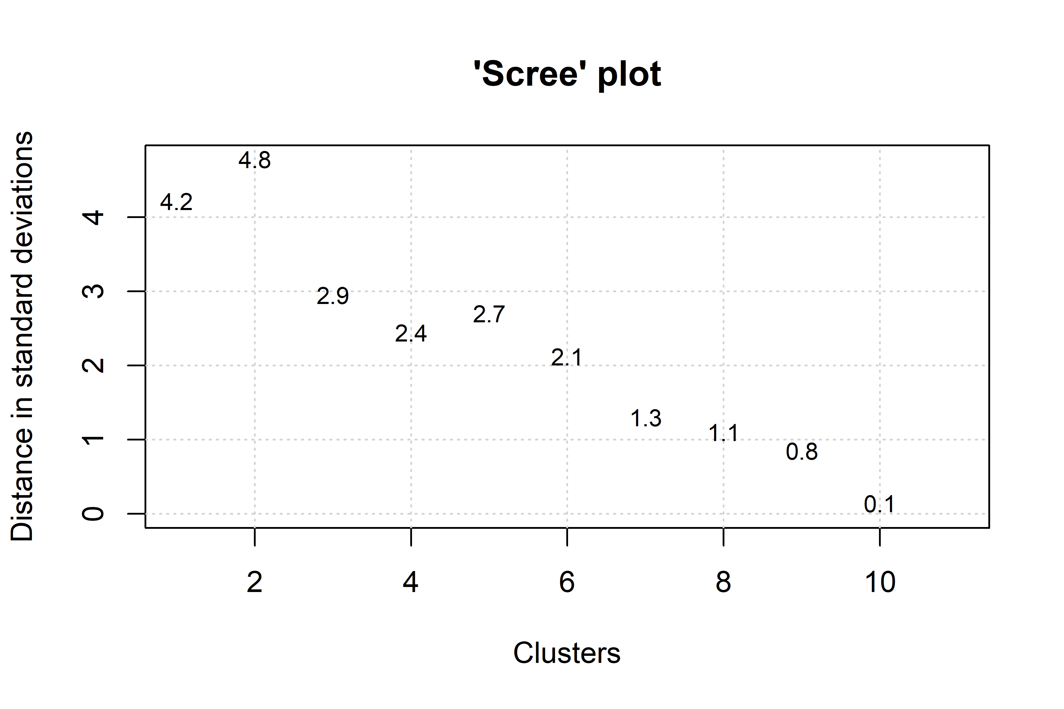
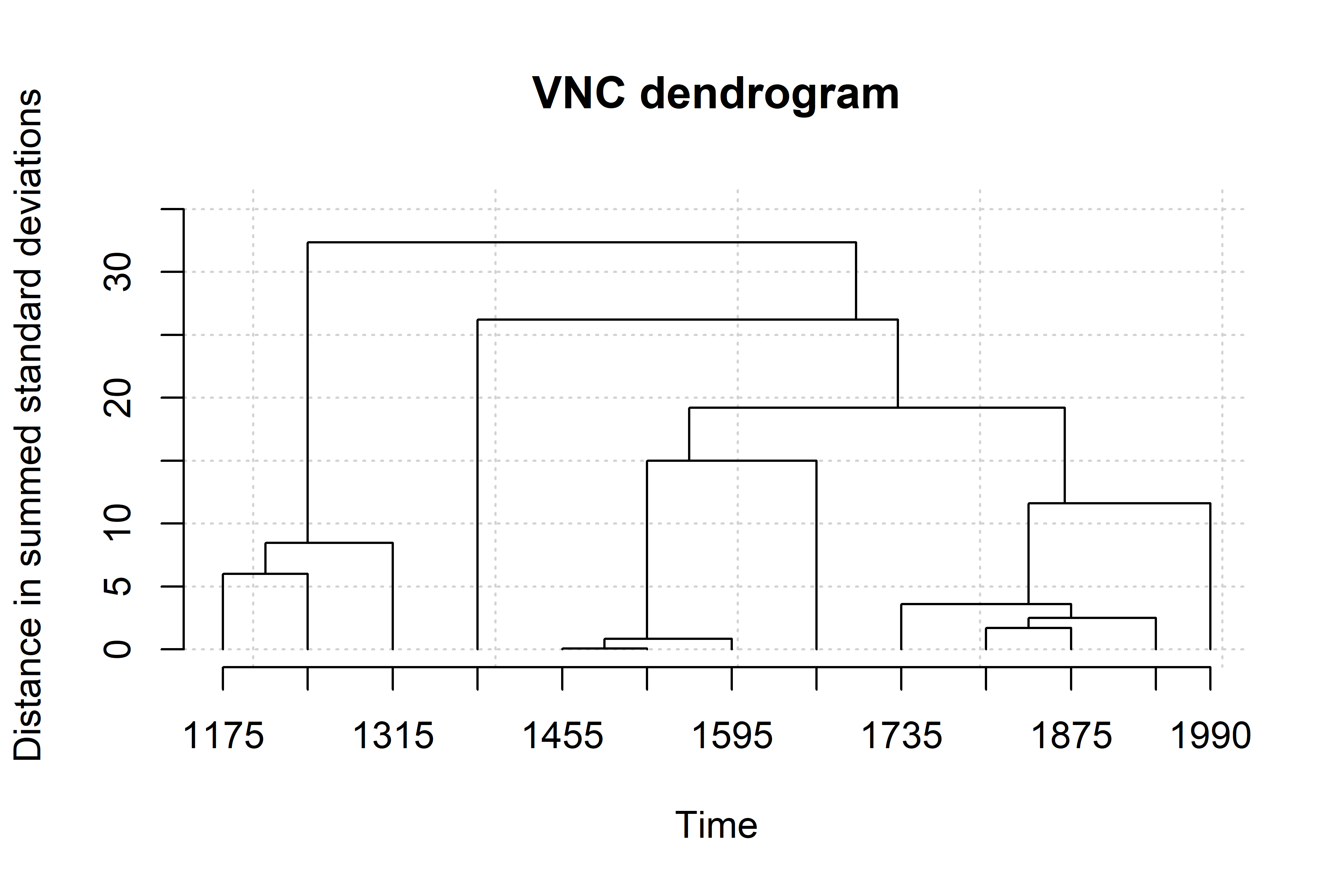
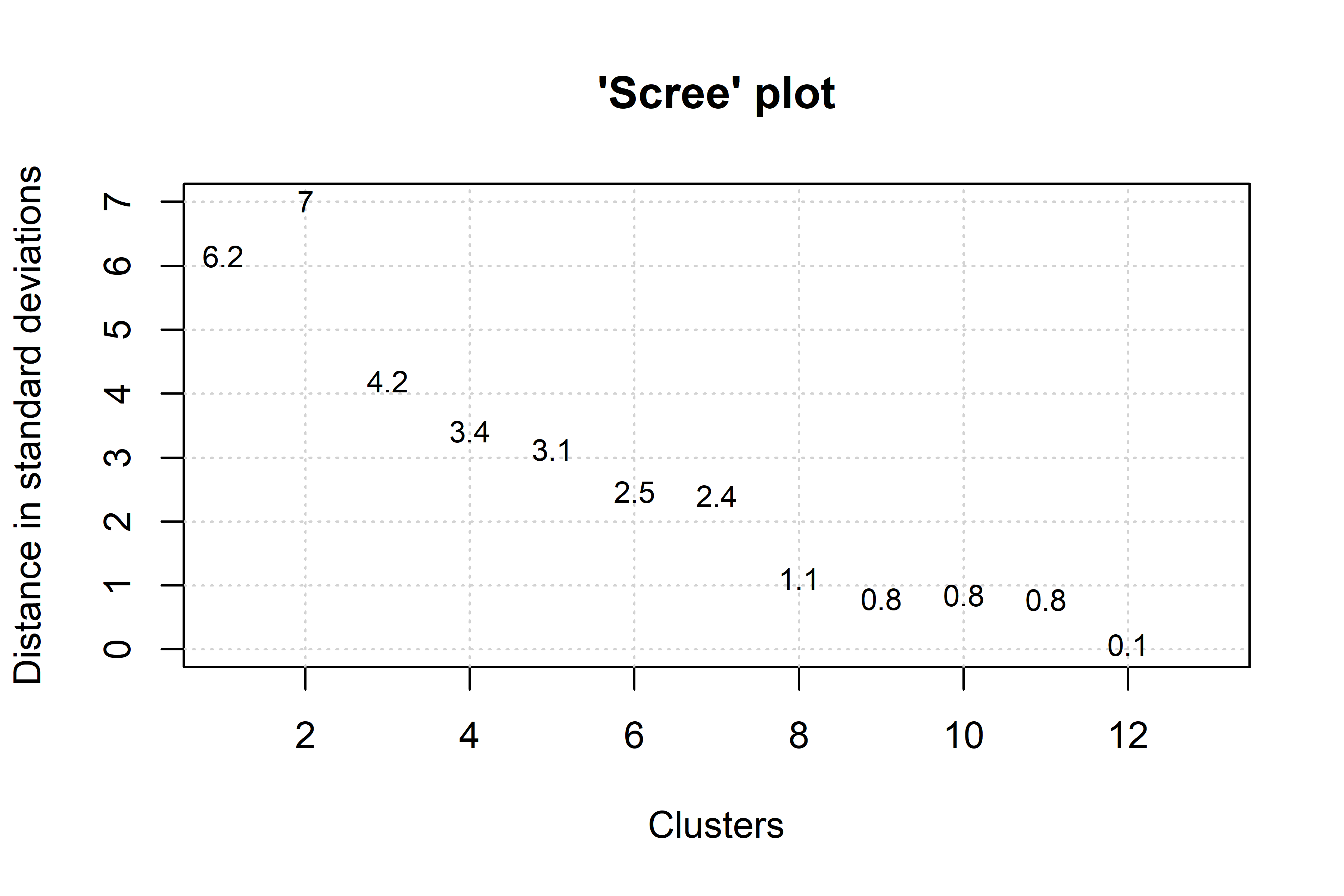
vnc.individual("VNC/ita_vnc_caus_70y.txt")Running the previous script will generate two graphs in separate windows: a dendrogram and a screeplot of the type shown below.
The dendogram specifies how periods are clustered (the periods that are the most similar are amalgamated first). The analyst should asses how many development stages are considered relevant to the diachronic study. The screeplot produced by the VNC function allows the linguist to decide by comparing the distances between successive mergers (measured with standard deviations). Essentially, one should observe the slope from left to right, and take the number of clusters with the largest differences, until the slope is leveled off (i.e., until the difference between clusters is marginal). In this case 4 or 6 clusters seems adequate. Given that we want to minimise data sparsity, we make the most parsimonious choice and select the first 4 clusters.
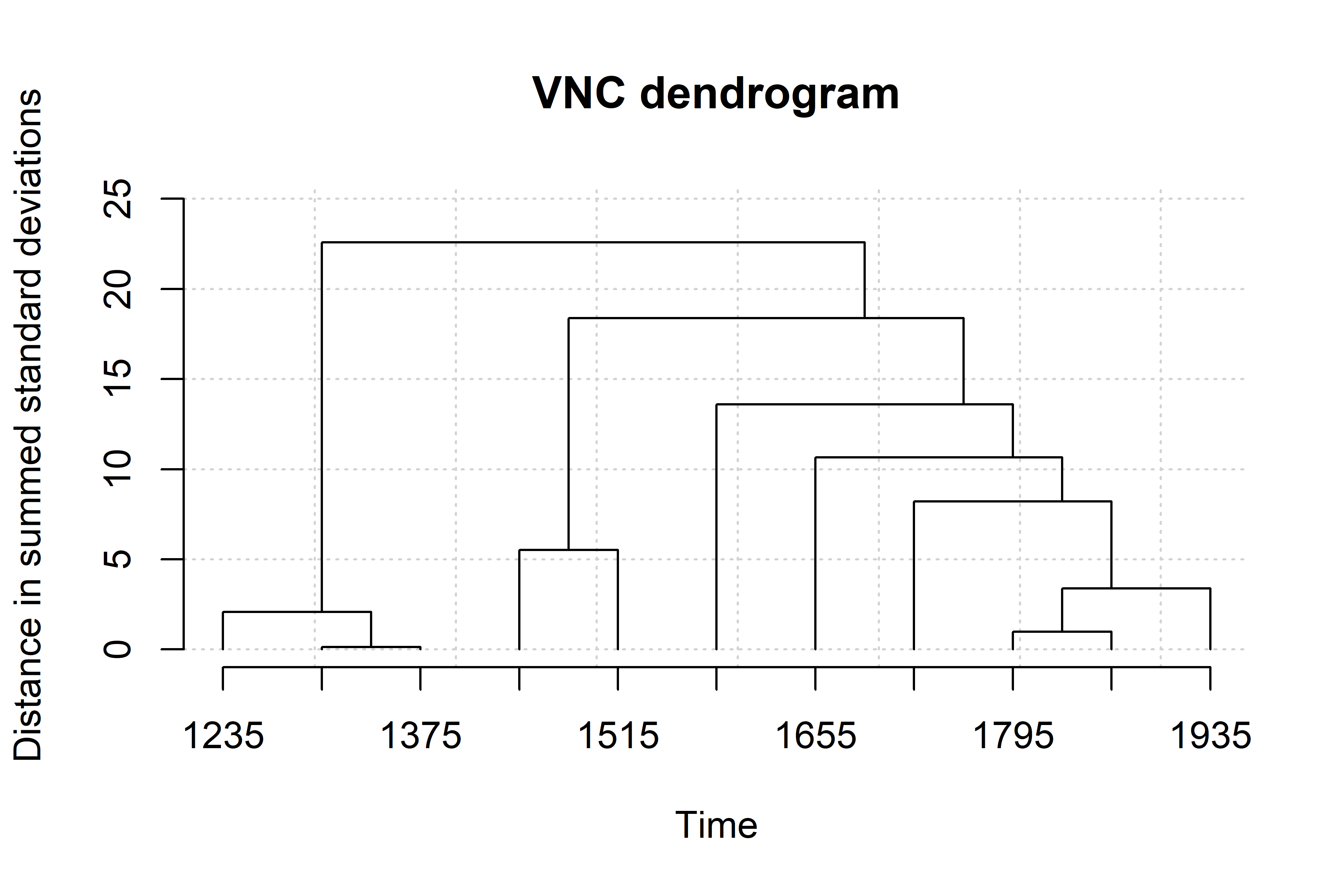
From the interpretation of the VNC results we end up with 4 significant periods for the development of the causal vs. non causal alternation in Spanish, dividing our dataset in the following periods: 1140-1209,1210-1279, 1280-1559, 1560-2001. Data are distributed across periods as summarised below. In Spanish causal uses are consistently higher than noncausal ones, but always below 60% except in the second period where they reach 73%.
esp<-esp %>%
  mutate(
    es_vnc70_apr25=case_when(
      year<1350 ~ "1140-1349",
      year<1420 ~ "1350-1419",
      year<1700 ~ "1420-1699",
      year<2002 ~ "1700-2001"
    )
  )

summary_es<-esp %>%
  group_by (es_vnc70_apr25, semantics) %>%
  summarise (n=n()) %>%
  mutate(rel.freq = paste0(round(100 * n/sum(n), 0), "%"))

summary_es %>%  kbl(booktabs = TRUE, col.names = c("VNC periods", "Semantics", "Count", "Relative Frequency (%)"), caption = "Spanish - Summary of the verb semantics by VNC periods") %>%
   collapse_rows(column = 1) %>%
kable_styling() | VNC periods | Semantics | Count | Relative Frequency (%) |
|---|---|---|---|
| 1140-1349 | caus | 434 | 55% |
| noncaus | 348 | 45% | |
| 1350-1419 | caus | 92 | 73% |
| noncaus | 34 | 27% | |
| 1420-1699 | caus | 1367 | 57% |
| noncaus | 1044 | 43% | |
| 1700-2001 | caus | 1653 | 52% |
| noncaus | 1523 | 48% |
For Italian, the relevant 4 periods indicated by the dendogram are 1200-1409, 1410-1549, 1550-1619 and 1620-1968, Data are distributed across periods as summarised below. In Italian, causal uses are consistently more frequent than non causal ones, always higher than 60%. Their relative frequency is at the highest in the second period, when they reach 73%, like in Spanish. However, the second VNC period in Italian is about a century later than in Spanish.
ita<-ita %>%
  mutate(
    ita_vnc70_apr25=case_when(
      year<1410 ~ "1200-1409",
      year<1550 ~ "1410-1549",
      year<1620 ~ "1550-1619",
      year<=1970 ~ "1620-1968"
    )
  )

summary_ita<-ita %>%
  group_by (ita_vnc70_apr25, semantics) %>%
  summarise (n=n()) %>%
  mutate(rel.freq = paste0(round(100 * n/sum(n), 0), "%"))

summary_ita %>%  kbl(booktabs = TRUE, col.names = c("VNC periods", "Semantics", "Count", "Relative Frequency (%)"), caption = "Italian - Summary of the verb semantics by VNC periods") %>%
   collapse_rows(column = 1) %>%
kable_styling() | VNC periods | Semantics | Count | Relative Frequency (%) |
|---|---|---|---|
| 1200-1409 | caus | 768 | 64% |
| noncaus | 441 | 36% | |
| 1410-1549 | caus | 1135 | 73% |
| noncaus | 421 | 27% | |
| 1550-1619 | caus | 695 | 67% |
| noncaus | 335 | 33% | |
| 1620-1968 | caus | 2700 | 62% |
| noncaus | 1635 | 38% |
Calculate the Causalness Degree
Once we found out the significant periods for the causal/non causal alternation, we calculate the share of causal uses by verb lemma and by period. Namely, every verb lemma in each of the four periods is assigned a number between 0 and 1, indicating the proportion (%) of causal uses vs. non causal uses. The table below summarises the distribution of causal uses by lemma and period (variable caus_use).
Italian:
caus_use_ita<-ita %>%
  group_by (ita_vnc70_apr25, lemma, semantics) %>%
  summarise (n=n()) %>%
  mutate(caus_use_ita_apr25 = n/sum(n))


caus_use_ita<-caus_use_ita %>% filter(semantics=="caus") %>% ungroup() %>% select (-semantics)

caus_use_ita %>% DT::datatable(rownames=F, filter="top")
Spanish:
caus_use_es <-esp %>%
  group_by (es_vnc70_apr25, lemma, semantics) %>%
  summarise (n=n()) %>%
  mutate(caus_use_es_apr25 = n/sum(n))


caus_use_es<-caus_use_es %>% filter(semantics=="caus") %>% ungroup() %>% select (-semantics)

caus_use_es %>% DT::datatable(rownames=F, filter="top")
And finally rejoin the individual languages new information (period70, vnc and causalness degree) to the main dataset:
# 1. Join caus_use_ita to ita by vnc and lemma
ita <- ita %>%
  left_join(caus_use_ita, by = c("ita_vnc70_apr25" = "ita_vnc70_apr25", "lemma" = "lemma"))

# 2. Join caus_use_es to esp by vnc and lemma
esp <- esp %>%
  left_join(caus_use_es, by = c("es_vnc70_apr25" = "es_vnc70_apr25", "lemma" = "lemma"))

names(ita)[duplicated(names(ita))]character(0)# 3. Rename columns to match target names before merging into romall
ita <- ita %>%
select(-any_of(c("vnc_period_apr25", "causalness_degree_apr25"))) %>%
rename(
vnc_period_apr25 = ita_vnc70_apr25,
causalness_degree_apr25 = caus_use_ita_apr25
)
esp <- esp %>%
select(-any_of(c("vnc_period_apr25", "causalness_degree_apr25"))) %>%
rename(
vnc_period_apr25 = es_vnc70_apr25,
causalness_degree_apr25 = caus_use_es_apr25
)
# 4. Bind the two enriched subsets together
combined <- bind_rows(ita, esp)
# 5. Join back to romall by id and lemma
romall <- romall %>%
select(-any_of(c("vnc_period_apr25", "causalness_degree_apr25"))) %>%
left_join(combined %>% select(id, lemma, vnc_period_apr25, causalness_degree_apr25),
by = c("id", "lemma"))
nc <- nc %>%
select(-any_of(c("vnc_period_apr25", "causalness_degree_apr25"))) %>%
left_join(combined %>% select(id, lemma, vnc_period_apr25, causalness_degree_apr25),
by = c("id", "lemma"))#only run this if you want to save the results of the VNC in a new xlsx file
openxlsx::write.xlsx(romall, "romall_new_VNC.xlsx")
openxlsx::write.xlsx(nc, "noncaus_new_VNC.xlsx")Diachronic analysis of the noncausal usage and causalness degree correlation
After calculating the diachronic causalness degree, we follow the procedure outlined in Heidinger (2015). For each verb in the two languages, we measure its correlation with the percentage of anticausative marking, iterating the count separately for each of the four periods. The results are shown in Figure 6 and Figure 7:
##Calculate causalness degree by language and period

caus_degree_ita <- romall %>%
  filter (language == 'italian') %>%
  group_by(meaning, vnc_period_apr25) %>%
  summarise(caus_degree = sum(semantics == 'caus') * 100 / n())

caus_degree_es <- romall %>%
  filter (language == 'spanish') %>%
  group_by(meaning, vnc_period_apr25) %>%
  summarise(caus_degree = sum(semantics == 'caus') * 100 / n())

##Calculate percentage of anticausative marking by language and period

coding_percentages_ita <- romall %>%
  group_by(meaning, semantics, coding, vnc_period_apr25) %>%
  filter (language == 'italian') %>%
  summarise(count = n()) %>%
  spread(coding, count, fill = 0) %>%
  mutate(caus_degree_vs_zero = caus * 100 / (caus + zero),
         prop_antic_vs_zero = antic * 100 / (antic + zero))


coding_percentages_es <- romall %>%
  group_by(meaning, semantics, coding, vnc_period_apr25) %>%
  filter (language == 'spanish') %>%
  summarise(count = n()) %>%
  spread(coding, count, fill = 0) %>%
  mutate(caus_degree_vs_zero = caus * 100 / (caus + zero),
         prop_antic_vs_zero = antic * 100 / (antic + zero))

##Scatter Plot of correlations between causalness degree and anticausative marking by period and language

merged_data_ita <- merge(caus_degree_ita, coding_percentages_ita, by = c("meaning", "vnc_period_apr25"))

merged_data_ita_noncaus <- merged_data_ita %>%
  filter(semantics == 'noncaus')

merged_data_ita_noncaus_1 <- merged_data_ita_noncaus %>%
  filter(vnc_period_apr25 == '1200-1409')

merged_data_ita_noncaus_2 <- merged_data_ita_noncaus %>%
  filter(vnc_period_apr25 == '1410-1549')

merged_data_ita_noncaus_3 <- merged_data_ita_noncaus %>%
  filter(vnc_period_apr25 == '1550-1619')

merged_data_ita_noncaus_4 <- merged_data_ita_noncaus %>%
  filter(vnc_period_apr25 == '1620-1968')

merged_data_es <- merge(caus_degree_es, coding_percentages_es, by = c("meaning", "vnc_period_apr25"))

merged_data_es_noncaus <- merged_data_es %>%
  filter(semantics == 'noncaus')

merged_data_es_noncaus_1 <- merged_data_es_noncaus %>%
  filter(vnc_period_apr25 == '1140-1349')

merged_data_es_noncaus_2 <- merged_data_es_noncaus %>%
  filter(vnc_period_apr25 == '1350-1419')

merged_data_es_noncaus_3 <- merged_data_es_noncaus %>%
  filter(vnc_period_apr25 == '1420-1699')

merged_data_es_noncaus_4 <- merged_data_es_noncaus %>%
  filter(vnc_period_apr25 == '1700-2001')

plot_ita_1 <- ggplot(merged_data_ita_noncaus_1, aes(x = caus_degree, y = prop_antic_vs_zero, label = meaning)) +
  geom_point() +
  labs(x = "Causalness",
       y = "%anticausative", title = "1200-1409") +
  theme_minimal() +
  theme(text = element_text(size = 14))

plot_ita_2 <- ggplot(merged_data_ita_noncaus_2, aes(x = caus_degree, y = prop_antic_vs_zero, label = meaning)) +
  geom_point() +
  labs(x = "Causalness",
       y = "%anticausative", title = "1410-1549") +
  theme_minimal() +
  theme(text = element_text(size = 14))

plot_ita_3 <- ggplot(merged_data_ita_noncaus_3, aes(x = caus_degree, y = prop_antic_vs_zero, label = meaning)) +
  geom_point() +
  labs(x = "Causalness",
       y = "%anticausative", title = "1550-1619") +
  theme_minimal() +
  theme(text = element_text(size = 14))

plot_ita_4 <- ggplot(merged_data_ita_noncaus_4, aes(x = caus_degree, y = prop_antic_vs_zero, label = meaning)) +
  geom_point() +
  labs(x = "Causalness",
       y = "%anticausative", title = "1620-1968") +
  theme_minimal() +
  theme(text = element_text(size = 14))

grid.arrange(plot_ita_1, plot_ita_2, plot_ita_3, plot_ita_4, nrow = 2, ncol = 2,  top = "Italian Correlation Plot")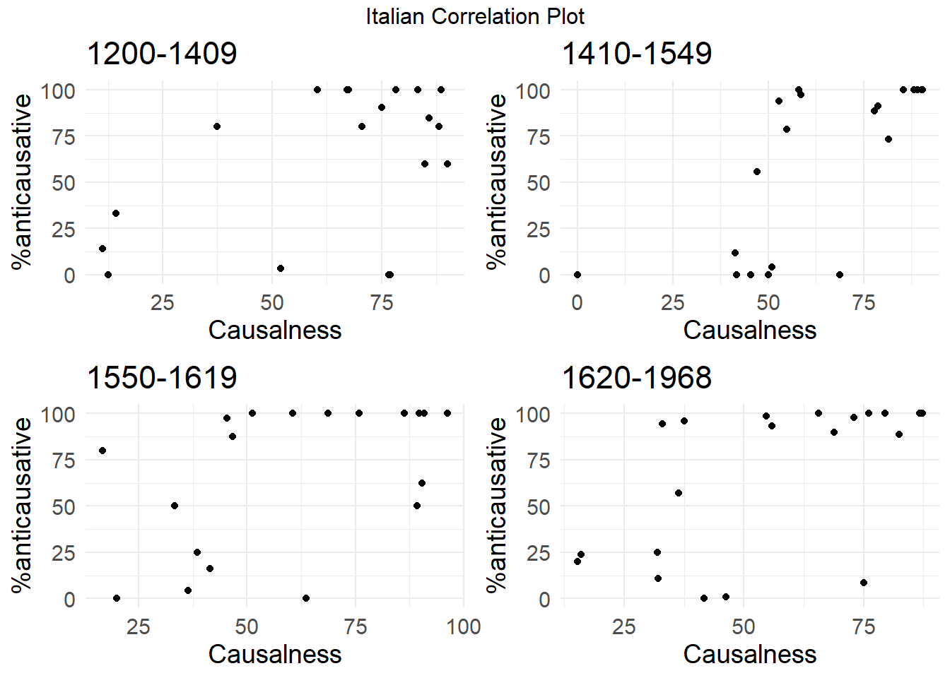
##Script for Figure 7
plot_es_1 <- ggplot(merged_data_es_noncaus_1, aes(x = caus_degree, y = prop_antic_vs_zero, label = meaning)) +
  geom_point() +
  labs(x = "Causalness",
       y = "%anticausative", title = "1140-1349") +
  theme_minimal() +
  theme(text = element_text(size = 14))

plot_es_2 <- ggplot(merged_data_es_noncaus_2, aes(x = caus_degree, y = prop_antic_vs_zero, label = meaning)) +
  geom_point() +
  labs(x = "Causalness",
       y = "%anticausative", title = "1350-1419") +
  theme_minimal() +
  theme(text = element_text(size = 14))

plot_es_3 <- ggplot(merged_data_es_noncaus_3, aes(x = caus_degree, y = prop_antic_vs_zero, label = meaning)) +
  geom_point() +
  labs(x = "Causalness",
       y = "%anticausative", title = "1420-1699") +
  theme_minimal() +
  theme(text = element_text(size = 14))

plot_es_4 <- ggplot(merged_data_es_noncaus_4, aes(x = caus_degree, y = prop_antic_vs_zero, label = meaning)) +
  geom_point() +
  labs(x = "Causalness",
       y = "%anticausative", title = "1700-2001") +
  theme_minimal() +
  theme(text = element_text(size = 14))

grid.arrange(plot_es_1, plot_es_2, plot_es_3, plot_es_4, nrow = 2, ncol = 2,  top = "Spanish Correlation Plot")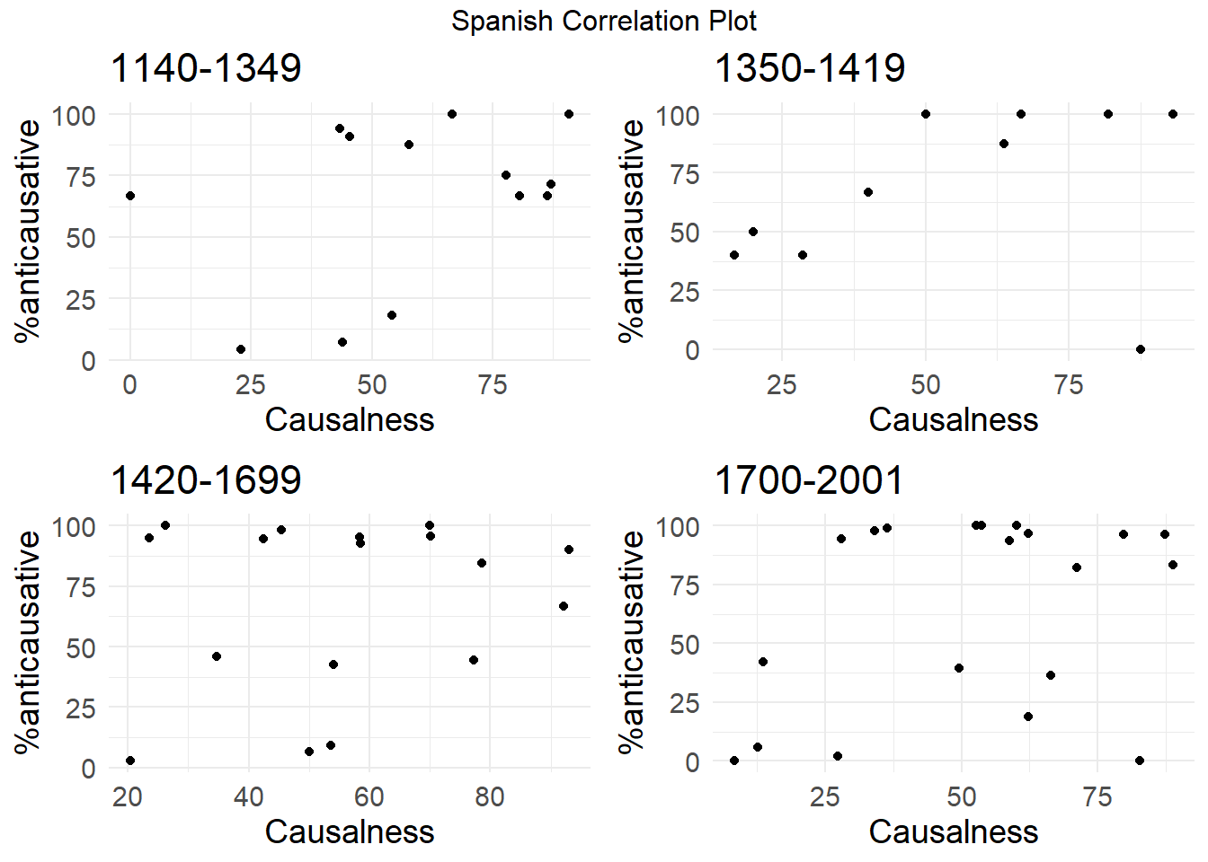
The corresponding correlation measures (Spearman Correlation Coefficient, SCC), alongside with p-values and the number of tokens analyzed for each period are given in the tables below:
## Function to format the p-values
format_pval <- function(p) {
  case_when(
    p < 0.001 ~ "< 0.001***",
    p < 0.01  ~ "< 0.01**",
    p < 0.05  ~ "< 0.05*",
    TRUE      ~ paste0("= ", round(p, 2))
  )
}

# Italian

## Individual periods datasets for Italian
datasets <- list(
  Period1 = merged_data_ita_noncaus_1,
  Period2 = merged_data_ita_noncaus_2,
  Period3 = merged_data_ita_noncaus_3,
  Period4 = merged_data_ita_noncaus_4
)

## Make a dataframe with the Spearman correlation and p-values
cor_table_ita <- purrr::imap_dfr(datasets, function(df, period) {
  test_result <- cor.test(df$caus_degree, df$prop_antic_vs_zero, method = "spearman", exact = FALSE)

  tibble(
    Period = period,
    Spearman_Correlation = round(test_result$estimate, 2),
    P_value = format_pval(test_result$p.value)
  )
})

## Show with kableExtra
cor_table_ita %>%
  kable("html", caption = "Italian - Spearman Correlation Between Causalness Degree and Anticausative Usage by Period") %>%
kable_styling(full_width = FALSE, bootstrap_options = c("striped", "hover", "condensed"))| Period | Spearman_Correlation | P_value |
|---|---|---|
| Period1 | 0.28 | = 0.24 |
| Period2 | 0.79 | < 0.001*** |
| Period3 | 0.58 | < 0.01** |
| Period4 | 0.59 | < 0.01** |
# Spanish

## Individual periods datasets for Italian
datasets_es <- list(
  Period1 = merged_data_es_noncaus_1,
  Period2 = merged_data_es_noncaus_2,
  Period3 = merged_data_es_noncaus_3,
  Period4 = merged_data_es_noncaus_4
)

## Make a dataframe with the Spearman correlation and p-values
cor_table_es <- purrr::imap_dfr(datasets_es, function(df, period) {
  test_result <- cor.test(df$caus_degree, df$prop_antic_vs_zero, method = "spearman", exact = FALSE)

  tibble(
    Period = period,
    Spearman_Correlation = round(test_result$estimate, 2),
    P_value = format_pval(test_result$p.value)
  )
})

## Show with KableExtra
cor_table_es %>%
  kable("html", caption = "Spearman Correlation Between Causalness and Anticausative Usage by Period (Spanish)") %>%
kable_styling(full_width = FALSE, bootstrap_options = c("striped", "hover", "condensed"))| Period | Spearman_Correlation | P_value |
|---|---|---|
| Period1 | 0.36 | = 0.22 |
| Period2 | 0.43 | = 0.19 |
| Period3 | 0.04 | = 0.88 |
| Period4 | 0.15 | = 0.52 |
Lexical or semantic effects?
The correlations discussed above are based on verb meaning, but we maintain that it is important to also discuss lemma-effects.
In particular, if the degree of causalness were a direct consequence of the degree of spontaneity of the event (Heidinger 2015), we would expect verbs that lexicalize the same event (and therefore presumably share the same degree of spontaneity) to have substantially the same causalness degree. We have verified whether this is the case by looking at the Italian data for period IV.
# Step 1: Calculate causal degree for Italian lemmas
caus_degree_ita_lemma <- romall %>%
  filter(language == "italian") %>%
  group_by(lemma, vnc_period_apr25) %>%
  summarise(caus_degree = sum(semantics == "caus") * 100 / n(), .groups = "drop")

# Step 2: Calculate coding percentages
coding_percentages_ita_lemma <- romall %>%
  filter(language == "italian") %>%
  group_by(lemma, semantics, coding, vnc_period_apr25) %>%
  summarise(count = n(), .groups = "drop") %>%
  pivot_wider(names_from = coding, values_from = count, values_fill = 0) %>%
  mutate(
    caus_degree_vs_zero = caus * 100 / (caus + zero),
    caus_degree_vs_zero = antic * 100 / (antic + zero)
  )

# Step 3: Merge the datasets
merged_data_ita_lemma <- left_join(
  caus_degree_ita_lemma,
  coding_percentages_ita_lemma,
  by = c("lemma", "vnc_period_apr25")
)

# Step 4: Filter for noncausative semantics and specific time period
merged_data_ita_noncaus_4_lemma <- merged_data_ita_lemma %>%
  filter(semantics == "noncaus", vnc_period_apr25 == "1620-1968")

# Step 5: Create verb meaning groups
groupings <- list(
  burn = c("ardere", "bruciare"),
  fill = c("empiere", "riempire"),
  melt = c("sciogliere", "fondere"),
  rise = c("alzare", "sollevare"),
  rock = c("dondolare", "oscillare"),
  split = c("dividere", "separare"),
  stop = c("arrestare", "fermare")
  )

# Assign group labels
merged_data_ita_noncaus_4_lemma <- merged_data_ita_noncaus_4_lemma %>%
  mutate(group = map_chr(lemma, function(l) {
    matched_group <- names(keep(groupings, ~ l %in% .x))
    if (length(matched_group) > 0) matched_group else NA_character_
  })) %>%
  filter(!is.na(group)) %>%
  mutate(group = factor(group, levels = names(groupings)))

# Step 6: Plot
ggplot(merged_data_ita_noncaus_4_lemma, aes(
  x = caus_degree,
  y = caus_degree_vs_zero,
  label = lemma,
  color = group,
  fill = group
)) +
  geom_point() +
  geom_text_repel(
    data = merged_data_ita_noncaus_4_lemma %>%
      filter(lemma %in% unlist(groupings)),
    aes(color = group),
    hjust = 0.5,
    vjust = -0.5,
    size = 4
  ) +
  labs(
    x = "Causalness",
    y = "% Anticausative"
  ) +
  theme_minimal() +
  theme(text = element_text(size = 14)) +
  scale_color_manual(
    name = "Meaning",
    values = c(
      burn = "red", fill = "blue", melt = "purple", rise = "brown",
      rock = "green", split = "cyan", stop = "orange"
    )
  ) +
  scale_fill_manual(
    name = "Meaning",
    values = c(
      burn = "red", fill = "blue", melt = "purple", rise = "brown",
      rock = "green", split = "cyan", stop = "orange"
    )
  ) +
  guides(color = guide_legend(override.aes = list(shape = 16, size = 4)))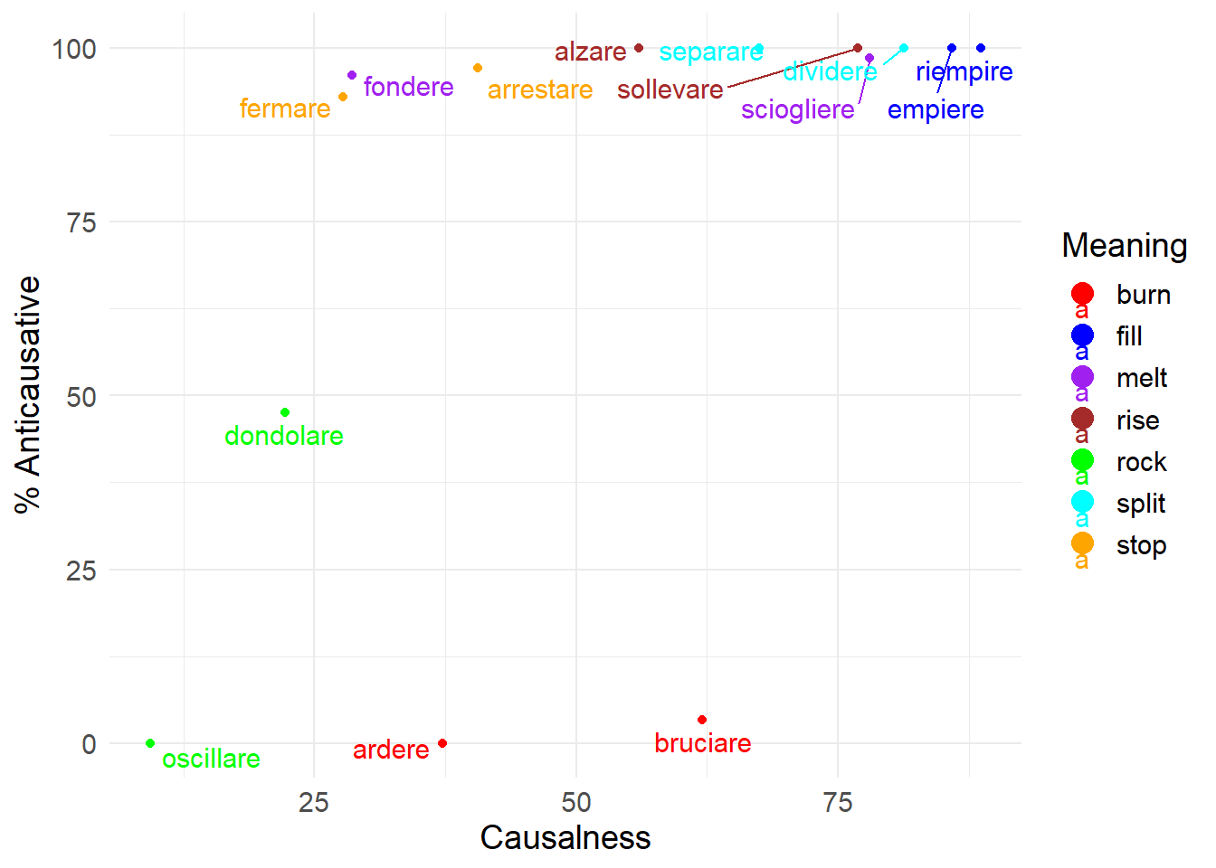
Part II: Frequency effects of causal degree on anticausative marking over time
# only non causal, verbs with categorical selection removed

ita_nc<-nc %>% filter(language=="italian")
es_nc<-nc %>% filter(language=="spanish")

ita_nc<-ita_nc %>% select(id, coding, meaning, lemma, vnc_period_apr25, causalness_degree_apr25)

ita_nc<-ita_nc %>% rename(period=vnc_period_apr25, causalness_degree=causalness_degree_apr25)

es_nc<-es_nc %>% select(id, coding, meaning, lemma, vnc_period_apr25, causalness_degree_apr25)

es_nc<-es_nc %>% rename(period=vnc_period_apr25, causalness_degree=causalness_degree_apr25)
Italian data: prepare for Beta Regression
Subset the Italian data to obtain unique combinations of lemma and period.
- Step 1: Aggregate data to calculate the proportion of anticausative codings
ita_agg <- ita_nc %>%
  group_by(lemma, period) %>%
  summarise(
    anticausative_count = sum(coding == "antic"),
    total_count = n(),
    proportion_anticausative = anticausative_count / total_count,
    causalness_degree = first(causalness_degree),
      ) %>%
ungroup()- Step 2: Create a lagged causalness_degree variable
ita_agg <- ita_agg %>%
  arrange(lemma, period) %>%
  group_by(lemma) %>%
  mutate(causalness_lagged = lag(causalness_degree)) %>%
  ungroup() %>%
  # Remove rows without previous causalness_degree (period 1)
  filter(!is.na(causalness_lagged))
Spanish data: prepare for Beta Regression
Subset the Spanish data to obtain unique combinations of lemma and period.
- Step 1: Aggregate data to calculate the proportion of anticausative codings:
es_agg <- es_nc %>%
  group_by(lemma, period) %>%
  summarise(
    anticausative_count = sum(coding == "antic"),
    total_count = n(),
    proportion_anticausative = anticausative_count / total_count,
    causalness_degree = first(causalness_degree),
    ) %>%
ungroup()- Step 2: Create a lagged causalness_degree variable:
es_agg <- es_agg %>%
  arrange(lemma, period) %>%
  group_by(lemma) %>%
  mutate(causalness_lagged = lag(causalness_degree)) %>%
  ungroup() %>%
  # Remove rows without previous causalness_degree (period 1)
  filter(!is.na(causalness_lagged))
Fit the Beta Regression model
Prepare the data for the regression model
- Step 1: join the Italian and Spanish sub-dataset
- Step 2: make the categorical variable into factors; transform
periodinto a numeric variable to be able to use it as a smooth term - Step 3: handling proportions for beta regression and adjust the numeric variables
In our data, the dependent variable proportion_anticausative takes values between 0 and 1. However, some observations are exactly 0 or 1. This poses a problem for beta regression (and its GAM extension with family = betar), because the beta distribution is only defined on the open interval (0,1).
To address this, we applied a small adjustment:
We created a copy of the original variable (proportion_anticausative_notadj) to preserve the raw values, including 0s and 1s.
We replaced the original proportion_anticausative with a slightly modified version where values equal to 0 are nudged to a very small positive number (ε = 0.000001), and values equal to 1 are nudged to just below 1 (1 – ε).
This ensures that all proportions are strictly within (0,1), making them suitable for beta regression, while still preserving the original variable for transparency and reference.
# Step 1
## Add a column to each dataset to distinguish them
italian <- ita_agg %>%
  mutate(language = "Italian")

spanish <- es_agg %>%
  mutate(language = "Spanish")

## Combine the datasets using bind_rows()
join <- bind_rows(italian, spanish)
# Step 2: prepare factors variables
join$language<-as.factor(join$language)
join$period_cat<-as.factor(join$period)
join$period<-as.factor(join$period)
join$period <- as.numeric(join$period_cat)
# Step 3: adjust the numeric variables to avoid exact 0s and 1s in the dependent variable and to make NAs into 0s for the predictors
epsilon <- 1e-6 # small adjustment so values fall strictly in (0,1)
join <- join %>%
mutate(
causalness_degree = ifelse(is.na(causalness_degree), 0, causalness_degree),
causalness_lagged = ifelse(is.na(causalness_lagged), 0, causalness_lagged),
proportion_anticausative_notadj = proportion_anticausative, # keep original
proportion_anticausative = pmin(pmax(proportion_anticausative, epsilon), 1 - epsilon) # adjusted
)
# quick checks
range(join$proportion_anticausative_notadj, na.rm = TRUE) # should still show 0 and 1[1] 0 1range(join$proportion_anticausative, na.rm = TRUE) # should now be (0,1)[1] 0.000001 0.999999all(join$proportion_anticausative > 0 & join$proportion_anticausative < 1) # should be TRUE[1] TRUEHereby a summary of the dataset with only unique combinations of lemma and period and their anticausative count, proportion, synchronic and lagged causalness degree:
# Summarize the dataset

summary_table <- join %>%
  group_by(language, lemma, period_cat) %>%
  summarise(
    N_Antic = sum(anticausative_count, na.rm = TRUE),   # Total count of anticausatives
    N_Total = sum(total_count, na.rm = TRUE),             # Total count of all occurrences
    `%_Antic_adjusted` = proportion_anticausative * 100,           # Directly use the original proportion value
    Causalness_Degree = causalness_degree,                # Use the original value
    Causalness_Lagged = causalness_lagged                 # Use the original value
  ) %>%
  ungroup()  # Remove grouping

summary_table %>%
  kable("html", caption = "Summary Table of Anticausative Proportions by Language, Lemma, and Period") %>%
  kable_styling(bootstrap_options = c("striped", "hover"), full_width = F) %>%
  row_spec(0, bold = TRUE) %>%  # Optional: make the header row bold
collapse_rows(columns = c(1, 2), valign = "top") # Collapse the rows for language and lemma| language | lemma | period_cat | N_Antic | N_Total | %_Antic_adjusted | Causalness_Degree | Causalness_Lagged |
|---|---|---|---|---|---|---|---|
| Italian | affondare | 1410-1549 | 0 | 1 | 0.000100 | 0.5000000 | 0.1250000 |
| 1550-1619 | 1 | 2 | 50.000000 | 0.3333333 | 0.5000000 | ||
| 1620-1968 | 5 | 21 | 23.809524 | 0.1600000 | 0.3333333 | ||
| alzare | 1410-1549 | 14 | 16 | 87.500000 | 0.8181818 | 0.8214286 | |
| 1550-1619 | 32 | 32 | 99.999900 | 0.6404494 | 0.8181818 | ||
| 1620-1968 | 155 | 155 | 99.999900 | 0.5596591 | 0.6404494 | ||
| ardere | 1410-1549 | 4 | 95 | 4.210526 | 0.4946809 | 0.5161290 | |
| 1550-1619 | 2 | 67 | 2.985075 | 0.3557692 | 0.4946809 | ||
| 1620-1968 | 0 | 86 | 0.000100 | 0.3722628 | 0.3557692 | ||
| arrestare | 1410-1549 | 3 | 3 | 99.999900 | 0.7857143 | 0.1111111 | |
| 1550-1619 | 6 | 7 | 85.714286 | 0.5625000 | 0.7857143 | ||
| 1620-1968 | 101 | 104 | 97.115385 | 0.4057143 | 0.5625000 | ||
| bruciare | 1550-1619 | 1 | 3 | 33.333333 | 0.5000000 | 0.8750000 | |
| 1620-1968 | 1 | 30 | 3.333333 | 0.6202532 | 0.5000000 | ||
| chiudere | 1410-1549 | 11 | 15 | 73.333333 | 0.8148148 | 0.6739130 | |
| 1550-1619 | 4 | 4 | 99.999900 | 0.9090909 | 0.8148148 | ||
| 1620-1968 | 38 | 38 | 99.999900 | 0.8671329 | 0.9090909 | ||
| dividere | 1410-1549 | 14 | 14 | 99.999900 | 0.9034483 | 0.7826087 | |
| 1550-1619 | 14 | 14 | 99.999900 | 0.8271605 | 0.9034483 | ||
| 1620-1968 | 51 | 51 | 99.999900 | 0.8131868 | 0.8271605 | ||
| fermare | 1410-1549 | 43 | 46 | 93.478261 | 0.4888889 | 0.8000000 | |
| 1550-1619 | 35 | 35 | 99.999900 | 0.4262295 | 0.4888889 | ||
| 1620-1968 | 172 | 185 | 92.972973 | 0.2773438 | 0.4262295 | ||
| fondere | 1410-1549 | 1 | 1 | 99.999900 | 0.8333333 | 0.8235294 | |
| 1550-1619 | 0 | 2 | 0.000100 | 0.0000000 | 0.8333333 | ||
| gelare | 1620-1968 | 7 | 31 | 22.580645 | 0.2954545 | 0.5000000 | |
| girare | 1410-1549 | 4 | 34 | 11.764706 | 0.4137931 | 0.1125828 | |
| 1550-1619 | 5 | 31 | 16.129032 | 0.4150943 | 0.4137931 | ||
| 1620-1968 | 16 | 146 | 10.958904 | 0.3209302 | 0.4150943 | ||
| migliorare | 1410-1549 | 0 | 6 | 0.000100 | 0.4545455 | 0.7692308 | |
| 1550-1619 | 0 | 4 | 0.000100 | 0.6363636 | 0.4545455 | ||
| 1620-1968 | 2 | 23 | 8.695652 | 0.7500000 | 0.6363636 | ||
| radunare | 1410-1549 | 38 | 39 | 97.435897 | 0.5851064 | 0.6032609 | |
| 1550-1619 | 15 | 15 | 99.999900 | 0.6052632 | 0.5851064 | ||
| 1620-1968 | 69 | 72 | 95.833333 | 0.3513514 | 0.6052632 | ||
| riempire | 1410-1549 | 5 | 5 | 99.999900 | 0.8148148 | 0.8333333 | |
| 1550-1619 | 2 | 2 | 99.999900 | 0.8823529 | 0.8148148 | ||
| 1620-1968 | 13 | 13 | 99.999900 | 0.8859649 | 0.8823529 | ||
| rompere | 1410-1549 | 16 | 16 | 99.999900 | 0.9030303 | 0.8586957 | |
| 1550-1619 | 6 | 6 | 99.999900 | 0.8983051 | 0.9030303 | ||
| 1620-1968 | 31 | 35 | 88.571429 | 0.8241206 | 0.8983051 | ||
| sciogliere | 1410-1549 | 7 | 7 | 99.999900 | 0.9078947 | 0.9393939 | |
| 1550-1619 | 5 | 6 | 83.333333 | 0.9259259 | 0.9078947 | ||
| 1620-1968 | 66 | 67 | 98.507463 | 0.7803279 | 0.9259259 | ||
| seccare | 1410-1549 | 5 | 9 | 55.555556 | 0.4705882 | 0.7058824 | |
| 1550-1619 | 4 | 5 | 80.000000 | 0.1666667 | 0.4705882 | ||
| 1620-1968 | 4 | 7 | 57.142857 | 0.3636364 | 0.1666667 | ||
| spegnere | 1410-1549 | 31 | 35 | 88.571429 | 0.7784810 | 0.6716418 | |
| 1550-1619 | 2 | 4 | 50.000000 | 0.8918919 | 0.7784810 | ||
| 1620-1968 | 53 | 59 | 89.830508 | 0.6878307 | 0.8918919 | ||
| svegliare | 1410-1549 | 11 | 14 | 78.571429 | 0.5483871 | 0.3750000 | |
| 1550-1619 | 7 | 8 | 87.500000 | 0.4666667 | 0.5483871 | ||
| 1620-1968 | 57 | 61 | 93.442623 | 0.5579710 | 0.4666667 | ||
| unire | 1410-1549 | 16 | 16 | 99.999900 | 0.5789474 | 0.8333333 | |
| 1550-1619 | 38 | 38 | 99.999900 | 0.5128205 | 0.5789474 | ||
| 1620-1968 | 157 | 159 | 98.742138 | 0.5470085 | 0.5128205 | ||
| Spanish | abrir | 1350-1419 | 1 | 1 | 99.999900 | 0.5000000 | 0.9074074 |
| 1420-1699 | 9 | 10 | 90.000000 | 0.9295775 | 0.5000000 | ||
| 1700-2001 | 26 | 27 | 96.296296 | 0.8732394 | 0.9295775 | ||
| alzar | 1350-1419 | 3 | 4 | 75.000000 | 0.7777778 | 0.5901639 | |
| 1420-1699 | 32 | 39 | 82.051282 | 0.8088235 | 0.7777778 | ||
| 1700-2001 | 30 | 34 | 88.235294 | 0.6761905 | 0.8088235 | ||
| apagar | 1420-1699 | 22 | 23 | 95.652174 | 0.7012987 | 0.8750000 | |
| 1700-2001 | 116 | 116 | 99.999900 | 0.6013746 | 0.7012987 | ||
| cerrar | 1420-1699 | 6 | 9 | 66.666667 | 0.9217391 | 0.8064516 | |
| 1700-2001 | 15 | 18 | 83.333333 | 0.8875000 | 0.9217391 | ||
| congelar | 1700-2001 | 17 | 18 | 94.444444 | 0.2800000 | 0.4242424 | |
| derretir | 1420-1699 | 49 | 52 | 94.230769 | 0.5737705 | 0.5000000 | |
| 1700-2001 | 71 | 73 | 97.260274 | 0.3539823 | 0.5737705 | ||
| despertar | 1350-1419 | 2 | 5 | 40.000000 | 0.2857143 | 0.5416667 | |
| 1420-1699 | 8 | 88 | 9.090909 | 0.5368421 | 0.2857143 | ||
| 1700-2001 | 43 | 109 | 39.449541 | 0.4953704 | 0.5368421 | ||
| fundir | 1420-1699 | 12 | 12 | 99.999900 | 0.5862069 | 0.7857143 | |
| 1700-2001 | 24 | 24 | 99.999900 | 0.2941176 | 0.5862069 | ||
| girar | 1420-1699 | 1 | 15 | 6.666667 | 0.5000000 | 0.4000000 | |
| 1700-2001 | 6 | 305 | 1.967213 | 0.2738095 | 0.5000000 | ||
| hervir | 1420-1699 | 4 | 148 | 2.702703 | 0.2043011 | 0.4400000 | |
| 1700-2001 | 7 | 118 | 5.932203 | 0.1259259 | 0.2043011 | ||
| hundir | 1700-2001 | 99 | 100 | 99.000000 | 0.3630573 | 0.2448980 | |
| juntar | 1350-1419 | 2 | 2 | 99.999900 | 0.5000000 | 0.6666667 | |
| 1420-1699 | 157 | 160 | 98.125000 | 0.4539249 | 0.5000000 | ||
| 1700-2001 | 26 | 26 | 99.999900 | 0.5272727 | 0.4539249 | ||
| levantar | 1350-1419 | 4 | 4 | 99.999900 | 0.0000000 | 0.1803279 | |
| 1700-2001 | 77 | 80 | 96.250000 | 0.5348837 | 0.3783784 | ||
| llenar | 1700-2001 | 27 | 28 | 96.428571 | 0.7971014 | 0.7000000 | |
| mejorar | 1350-1419 | 2 | 5 | 40.000000 | 0.1666667 | 0.2287582 | |
| 1420-1699 | 17 | 40 | 42.500000 | 0.5402299 | 0.1666667 | ||
| 1700-2001 | 9 | 48 | 18.750000 | 0.6220472 | 0.5402299 | ||
| parar | 1350-1419 | 2 | 2 | 99.999900 | 0.8181818 | 0.5775862 | |
| 1420-1699 | 43 | 94 | 45.744681 | 0.3472222 | 0.8181818 | ||
| 1700-2001 | 16 | 38 | 42.105263 | 0.1363636 | 0.3472222 | ||
| quemar | 1350-1419 | 2 | 2 | 99.999900 | 0.9310345 | 0.8703704 | |
| 1420-1699 | 38 | 45 | 84.444444 | 0.7867299 | 0.9310345 | ||
| 1700-2001 | 14 | 17 | 82.352941 | 0.7118644 | 0.7867299 | ||
| romper | 1420-1699 | 16 | 36 | 44.444444 | 0.7721519 | 0.7777778 | |
| 1700-2001 | 19 | 52 | 36.538461 | 0.6645161 | 0.7721519 | ||
| secar | 1350-1419 | 2 | 4 | 50.000000 | 0.2000000 | 0.4333333 | |
| 1420-1699 | 76 | 76 | 99.999900 | 0.2621359 | 0.2000000 | ||
| 1700-2001 | 28 | 29 | 96.551724 | 0.6233766 | 0.2621359 |
Model fit and model selection
Hereby we fit a beta regression model with mgvc::gam: model1 is the maximal model which includes
s(causalness_degree, k=10), s(causalness_lagged, k=10) and s(period, k=5): global smooth terms — these model the overall nonlinear effects of each predictor across all languages.s(causalness_lagged, by = language, k = 10, bs = "cs", m = 1), s(causalness_degree, by = language, k = 10, bs = "cs", m = 1), ands(period, by = language, k = 5, bs = "cs", m= 1): group-wise smooths (by language) — these allow the shape of the smooth to differ between Italian and Spanish.family = betar(...): the model uses a beta regression family, designed for proportions or rates strictly between 0 and 1.link = "logit": the logit link function ensures predicted values remain within the (0, 1) range.method = "ML": the model is fitted using maximum likelihood estimation (ML) rather than the default restricted maximum likelihood (REML). ML is typically used when comparing models with different fixed-effect structures, since REML estimates are not directly comparable across models with different smooth terms.
model1 <- gam(
  proportion_anticausative ~
    s(causalness_lagged, k=10)+
    s(causalness_degree, k=10)+
    s(period, k=5)+
    s(causalness_lagged, by = language, k = 10, bs = "cs", m = 1) +
    s(causalness_degree, by = language, k = 10, bs = "cs", m = 1) +
    s(period, by = language, k = 5, bs = "cs", m= 1),
  family = betar(link = "logit"),
  data = join,
  method="ML"
)

# Summarize the model
summary(model1)
Family: Beta regression(0.536)
Link function: logit

Formula:
proportion_anticausative ~ s(causalness_lagged, k = 10) + s(causalness_degree,
    k = 10) + s(period, k = 5) + s(causalness_lagged, by = language,
    k = 10, bs = "cs", m = 1) + s(causalness_degree, by = language,
    k = 10, bs = "cs", m = 1) + s(period, by = language, k = 5,
    bs = "cs", m = 1)

Parametric coefficients:
            Estimate Std. Error z value Pr(>|z|)
(Intercept)   0.7087     0.1304   5.435 5.49e-08 ***
---
Signif. codes:  0 '***' 0.001 '**' 0.01 '*' 0.05 '.' 0.1 ' ' 1

Approximate significance of smooth terms:
                                           edf Ref.df Chi.sq p-value
s(causalness_lagged)                 1.000e+00      1  1.171 0.27928
s(causalness_degree)                 1.000e+00      1 11.195 0.00082 ***
s(period)                            1.000e+00      1  0.259 0.61071
s(causalness_lagged):languageItalian 7.500e-06      9  0.000 0.58048
s(causalness_lagged):languageSpanish 1.190e-04      9  0.000 0.59603
s(causalness_degree):languageItalian 1.088e-05      9  0.000 0.18367
s(causalness_degree):languageSpanish 1.299e+00      9  8.120 0.00261 **
s(period):languageItalian            7.832e-05      3  0.000 0.24791
s(period):languageSpanish            1.844e-05      3  0.000 0.21472
---
Signif. codes:  0 '***' 0.001 '**' 0.01 '*' 0.05 '.' 0.1 ' ' 1

R-sq.(adj) =  0.148   Deviance explained = 26.7%
-ML = -302.44 Scale est. = 1 n = 99- Step 3: Backward selection
In model2 we start by removing s(period, k=5)+, as it is the term with the highest pvalue. + anova(..., test="Chisq") compares two nested GAM models (e.g., model1 and a simpler model2) using a likelihood ratio test (Chi-squared test) + AIC(): it calculates the AIC of the two models, which is a measure of model fit that balances goodness-of-fit with model complexity (penalizes overfitting)
We continue removing terms with high p-value, until we reach the most parsimonious model.
The anova shows is ok to remove the term.
model2 <- gam(
  proportion_anticausative ~
    s(causalness_lagged, k=10)+
    s(causalness_degree, k=10)+
    #s(period, k=5)+
    s(causalness_lagged, by = language, k = 10, bs = "cs", m = 1) +
    s(causalness_degree, by = language, k = 10, bs = "cs", m = 1)+
    s(period, by = language, k = 5, bs = "cs", m= 1),
  family = betar(link = "logit"),
  data = join,
  method="ML"
)

# Summarize the model
summary(model2)
Family: Beta regression(0.536)
Link function: logit

Formula:
proportion_anticausative ~ s(causalness_lagged, k = 10) + s(causalness_degree,
    k = 10) + s(causalness_lagged, by = language, k = 10, bs = "cs",
    m = 1) + s(causalness_degree, by = language, k = 10, bs = "cs",
    m = 1) + s(period, by = language, k = 5, bs = "cs", m = 1)

Parametric coefficients:
            Estimate Std. Error z value Pr(>|z|)
(Intercept)   0.7104     0.1305   5.445 5.19e-08 ***
---
Signif. codes:  0 '***' 0.001 '**' 0.01 '*' 0.05 '.' 0.1 ' ' 1

Approximate significance of smooth terms:
                                           edf Ref.df Chi.sq  p-value
s(causalness_lagged)                 1.000e+00      1  1.129 0.288069
s(causalness_degree)                 1.000e+00      1 11.940 0.000549 ***
s(causalness_lagged):languageItalian 4.501e-06      9  0.000 0.623366
s(causalness_lagged):languageSpanish 7.298e-05      9  0.000 0.634162
s(causalness_degree):languageItalian 5.413e-06      9  0.000 0.188334
s(causalness_degree):languageSpanish 1.322e+00      9  8.454 0.002208 **
s(period):languageItalian            5.765e-05      3  0.000 0.514120
s(period):languageSpanish            1.327e-01      3  0.177 0.244040
---
Signif. codes:  0 '***' 0.001 '**' 0.01 '*' 0.05 '.' 0.1 ' ' 1

R-sq.(adj) =  0.161   Deviance explained = 26.8%
-ML = -302.32 Scale est. = 1 n = 99anova(model1, model2, test="Chisq")Analysis of Deviance Table
Model 1: proportion_anticausative ~ s(causalness_lagged, k = 10) + s(causalness_degree,
k = 10) + s(period, k = 5) + s(causalness_lagged, by = language,
k = 10, bs = "cs", m = 1) + s(causalness_degree, by = language,
k = 10, bs = "cs", m = 1) + s(period, by = language, k = 5,
bs = "cs", m = 1)
Model 2: proportion_anticausative ~ s(causalness_lagged, k = 10) + s(causalness_degree,
k = 10) + s(causalness_lagged, by = language, k = 10, bs = "cs",
m = 1) + s(causalness_degree, by = language, k = 10, bs = "cs",
m = 1) + s(period, by = language, k = 5, bs = "cs", m = 1)
Resid. Df Resid. Dev Df Deviance Pr(>Chi)
1 92.750 -609.35
2 93.361 -609.48 -0.61183 0.12349 AIC(model1, model2) df AIC
model1 6.774768 -595.8037
model2 6.046560 -597.3836In model3 we need to remove s(causalness_lagged, by = language, k = 10, bs = "cs", m = 1), as it is the term with the highest pvalue. Anova shows it’s not ok to remove.
model3 <- gam(
  proportion_anticausative ~
    s(causalness_lagged, k=10)+
    s(causalness_degree, k=10)+
    #s(period, k=5)+
    #s(causalness_lagged, by = language, k = 10, bs = "cs", m = 1) +
    s(causalness_degree, by = language, k = 10, bs = "cs", m = 1)+
    s(period, by = language, k = 5, bs = "cs", m= 1),
  family = betar(link = "logit"),
  data = join,
  method="ML"
)

# Summarize the model
summary(model3)
Family: Beta regression(0.536)
Link function: logit

Formula:
proportion_anticausative ~ s(causalness_lagged, k = 10) + s(causalness_degree,
    k = 10) + s(causalness_degree, by = language, k = 10, bs = "cs",
    m = 1) + s(period, by = language, k = 5, bs = "cs", m = 1)

Parametric coefficients:
            Estimate Std. Error z value Pr(>|z|)
(Intercept)   0.7104     0.1305   5.445 5.19e-08 ***
---
Signif. codes:  0 '***' 0.001 '**' 0.01 '*' 0.05 '.' 0.1 ' ' 1

Approximate significance of smooth terms:
                                           edf Ref.df Chi.sq  p-value
s(causalness_lagged)                 1.000e+00      1  1.129 0.288085
s(causalness_degree)                 1.000e+00      1 11.940 0.000549 ***
s(causalness_degree):languageItalian 7.061e-06      9  0.000 0.188330
s(causalness_degree):languageSpanish 1.322e+00      9  8.455 0.002208 **
s(period):languageItalian            1.505e-04      3  0.000 0.514117
s(period):languageSpanish            1.327e-01      3  0.177 0.244041
---
Signif. codes:  0 '***' 0.001 '**' 0.01 '*' 0.05 '.' 0.1 ' ' 1

R-sq.(adj) =  0.161   Deviance explained = 26.8%
-ML = -302.32 Scale est. = 1 n = 99anova(model3, model2, test="Chisq")Analysis of Deviance Table
Model 1: proportion_anticausative ~ s(causalness_lagged, k = 10) + s(causalness_degree,
k = 10) + s(causalness_degree, by = language, k = 10, bs = "cs",
m = 1) + s(period, by = language, k = 5, bs = "cs", m = 1)
Model 2: proportion_anticausative ~ s(causalness_lagged, k = 10) + s(causalness_degree,
k = 10) + s(causalness_lagged, by = language, k = 10, bs = "cs",
m = 1) + s(causalness_degree, by = language, k = 10, bs = "cs",
m = 1) + s(period, by = language, k = 5, bs = "cs", m = 1)
Resid. Df Resid. Dev Df Deviance Pr(>Chi)
1 93.361 -609.48
2 93.361 -609.48 -0.00015192 -9.173e-05 0.0007147 ***
---
Signif. codes: 0 '***' 0.001 '**' 0.01 '*' 0.05 '.' 0.1 ' ' 1AIC(model3, model2) df AIC
model3 6.046661 -597.3835
model2 6.046560 -597.3836We go back to model2 and in model4 we remove s(period, by = language, k = 5, bs = "cs", m= 1) which is the second next highest p-value. The comparison between model2 and model4 shows it is ok to remove this term.
model4 <- gam(
  proportion_anticausative ~
    s(causalness_lagged, k=10)+
    s(causalness_degree, k=10)+
    #s(period, k=5)+
    s(causalness_lagged, by = language, k = 10, bs = "cs", m = 1) +
    s(causalness_degree, by = language, k = 10, bs = "cs", m = 1),
    #s(period, by = language, k = 5, bs = "cs", m= 1),
  family = betar(link = "logit"),
  data = join,
  method="ML"
)
# Summarize the model
summary(model4)
Family: Beta regression(0.535)
Link function: logit

Formula:
proportion_anticausative ~ s(causalness_lagged, k = 10) + s(causalness_degree,
    k = 10) + s(causalness_lagged, by = language, k = 10, bs = "cs",
    m = 1) + s(causalness_degree, by = language, k = 10, bs = "cs",
    m = 1)

Parametric coefficients:
            Estimate Std. Error z value Pr(>|z|)
(Intercept)   0.7114     0.1304   5.456 4.86e-08 ***
---
Signif. codes:  0 '***' 0.001 '**' 0.01 '*' 0.05 '.' 0.1 ' ' 1

Approximate significance of smooth terms:
                                           edf Ref.df Chi.sq p-value
s(causalness_lagged)                 1.000e+00      1  1.177 0.27800
s(causalness_degree)                 1.000e+00      1  0.004 0.94653
s(causalness_lagged):languageItalian 2.142e-05      9  0.000 0.59328
s(causalness_lagged):languageSpanish 1.763e-05      9  0.000 0.60515
s(causalness_degree):languageItalian 1.345e+00      9  8.353 0.00243 **
s(causalness_degree):languageSpanish 1.203e-05      9  0.000 0.14713
---
Signif. codes:  0 '***' 0.001 '**' 0.01 '*' 0.05 '.' 0.1 ' ' 1

R-sq.(adj) =  0.162   Deviance explained = 26.4%
-ML = -302.15 Scale est. = 1 n = 99anova(model2, model4, test="Chisq")Analysis of Deviance Table
Model 1: proportion_anticausative ~ s(causalness_lagged, k = 10) + s(causalness_degree,
k = 10) + s(causalness_lagged, by = language, k = 10, bs = "cs",
m = 1) + s(causalness_degree, by = language, k = 10, bs = "cs",
m = 1) + s(period, by = language, k = 5, bs = "cs", m = 1)
Model 2: proportion_anticausative ~ s(causalness_lagged, k = 10) + s(causalness_degree,
k = 10) + s(causalness_lagged, by = language, k = 10, bs = "cs",
m = 1) + s(causalness_degree, by = language, k = 10, bs = "cs",
m = 1)
Resid. Df Resid. Dev Df Deviance Pr(>Chi)
1 93.361 -609.48
2 93.674 -609.11 -0.31242 -0.371 0.1941AIC(model2, model4) df AIC
model2 6.046560 -597.3836
model4 5.835506 -597.4347In model5 we need to remove s(causalness_degree, k=10), as it is only marginally significant. Anova shows that removing it does not affect the model.
model5 <- gam(
  proportion_anticausative ~
    s(causalness_lagged, k=10)+
    #s(causalness_degree, k=10)+
    #s(period, k=5)+
    s(causalness_lagged, by = language, k = 10, bs = "cs", m = 1) +
    s(causalness_degree, by = language, k = 10, bs = "cs", m = 1),
    #s(period, by = language, k = 5, bs = "cs", m= 1),
  family = betar(link = "logit"),
  data = join,
  method="ML"
)
# Summarize the model
summary(model5)
Family: Beta regression(0.535)
Link function: logit

Formula:
proportion_anticausative ~ s(causalness_lagged, k = 10) + s(causalness_lagged,
    by = language, k = 10, bs = "cs", m = 1) + s(causalness_degree,
    by = language, k = 10, bs = "cs", m = 1)

Parametric coefficients:
            Estimate Std. Error z value Pr(>|z|)
(Intercept)   0.7121     0.1300   5.476 4.34e-08 ***
---
Signif. codes:  0 '***' 0.001 '**' 0.01 '*' 0.05 '.' 0.1 ' ' 1

Approximate significance of smooth terms:
                                           edf Ref.df Chi.sq  p-value
s(causalness_lagged)                 1.000e+00      1  1.507 0.219630
s(causalness_lagged):languageItalian 6.165e-05      9  0.000 0.614137
s(causalness_lagged):languageSpanish 4.849e-05      9  0.000 0.623972
s(causalness_degree):languageItalian 1.401e+00      9 13.356 0.000165 ***
s(causalness_degree):languageSpanish 4.976e-05      9  0.000 0.673066
---
Signif. codes:  0 '***' 0.001 '**' 0.01 '*' 0.05 '.' 0.1 ' ' 1

R-sq.(adj) =  0.171   Deviance explained = 26.4%
-ML = -302.15 Scale est. = 1 n = 99anova(model4, model5, test="Chisq")Analysis of Deviance Table
Model 1: proportion_anticausative ~ s(causalness_lagged, k = 10) + s(causalness_degree,
k = 10) + s(causalness_lagged, by = language, k = 10, bs = "cs",
m = 1) + s(causalness_degree, by = language, k = 10, bs = "cs",
m = 1)
Model 2: proportion_anticausative ~ s(causalness_lagged, k = 10) + s(causalness_lagged,
by = language, k = 10, bs = "cs", m = 1) + s(causalness_degree,
by = language, k = 10, bs = "cs", m = 1)
Resid. Df Resid. Dev Df Deviance Pr(>Chi)
1 93.674 -609.11
2 94.713 -609.04 -1.039 -0.066054 0.8105AIC(model4, model5) df AIC
model4 5.835506 -597.4347
model5 4.844266 -599.3511The next candidate for removal is s(causalness_lagged) in model6 (as we tried already removing s(causalness_lagged, by = language, k = 10, bs = "cs", m = 1). It is not completely ok to remove that, because the anova is marginally significant and the AIC is lower for model5.
So we go back to model5 and this time in model7 we remove s(causalness_lagged, by = language, k = 10, bs = "cs", m = 1). It seems that model5 is our final model, as removing this group-wise smooth is not ok.
model6 <- gam(
  proportion_anticausative ~
    #s(causalness_lagged, k=10)+
    #s(causalness_degree, k=10)+
    #s(period, k=5)+
    s(causalness_lagged, by = language, k = 10, bs = "cs", m = 1) +
    s(causalness_degree, by = language, k = 10, bs = "cs", m = 1),
    #s(period, by = language, k = 5, bs = "cs", m= 1),
  family = betar(link = "logit"),
  data = join,
  method="ML"
)
# Summarize the model
summary(model6) #
Family: Beta regression(0.53)
Link function: logit

Formula:
proportion_anticausative ~ s(causalness_lagged, by = language,
    k = 10, bs = "cs", m = 1) + s(causalness_degree, by = language,
    k = 10, bs = "cs", m = 1)

Parametric coefficients:
            Estimate Std. Error z value Pr(>|z|)
(Intercept)   0.7051     0.1303   5.411 6.26e-08 ***
---
Signif. codes:  0 '***' 0.001 '**' 0.01 '*' 0.05 '.' 0.1 ' ' 1

Approximate significance of smooth terms:
                                           edf Ref.df Chi.sq  p-value
s(causalness_lagged):languageItalian 3.147e-01      9  0.476    0.199
s(causalness_lagged):languageSpanish 1.549e-04      9  0.000    0.553
s(causalness_degree):languageItalian 1.464e+00      9 16.542 1.06e-05 ***
s(causalness_degree):languageSpanish 5.403e-05      9  0.000    0.946
---
Signif. codes:  0 '***' 0.001 '**' 0.01 '*' 0.05 '.' 0.1 ' ' 1

R-sq.(adj) =  0.148   Deviance explained = 25.7%
-ML = -301.38 Scale est. = 1 n = 99anova(model6, model5, test="Chisq")Analysis of Deviance Table
Model 1: proportion_anticausative ~ s(causalness_lagged, by = language,
k = 10, bs = "cs", m = 1) + s(causalness_degree, by = language,
k = 10, bs = "cs", m = 1)
Model 2: proportion_anticausative ~ s(causalness_lagged, k = 10) + s(causalness_lagged,
by = language, k = 10, bs = "cs", m = 1) + s(causalness_degree,
by = language, k = 10, bs = "cs", m = 1)
Resid. Df Resid. Dev Df Deviance Pr(>Chi)
1 94.929 -608.43
2 94.713 -609.04 0.21632 0.60493 0.09856 .
---
Signif. codes: 0 '***' 0.001 '**' 0.01 '*' 0.05 '.' 0.1 ' ' 1AIC(model6, model5) df AIC
model6 4.424766 -599.5852
model5 4.844266 -599.3511model7 <- gam(
proportion_anticausative ~
s(causalness_lagged, k=10)+
#s(causalness_degree, k=10)+
#s(period, k=5)+
#s(causalness_lagged, by = language, k = 10, bs = "cs", m = 1) +
s(causalness_degree, by = language, k = 10, bs = "cs", m = 1),
#s(period, by = language, k = 5, bs = "cs", m= 1),
family = betar(link = "logit"),
data = join,
method="ML"
)
# Summarize the model
summary(model7) #
Family: Beta regression(0.535)
Link function: logit

Formula:
proportion_anticausative ~ s(causalness_lagged, k = 10) + s(causalness_degree,
    by = language, k = 10, bs = "cs", m = 1)

Parametric coefficients:
            Estimate Std. Error z value Pr(>|z|)
(Intercept)   0.7121     0.1300   5.476 4.34e-08 ***
---
Signif. codes:  0 '***' 0.001 '**' 0.01 '*' 0.05 '.' 0.1 ' ' 1

Approximate significance of smooth terms:
                                           edf Ref.df Chi.sq  p-value
s(causalness_lagged)                 1.000e+00      1  1.507 0.219621
s(causalness_degree):languageItalian 1.401e+00      9 13.356 0.000165 ***
s(causalness_degree):languageSpanish 8.654e-05      9  0.000 0.673050
---
Signif. codes:  0 '***' 0.001 '**' 0.01 '*' 0.05 '.' 0.1 ' ' 1

R-sq.(adj) =  0.171   Deviance explained = 26.4%
-ML = -302.15 Scale est. = 1 n = 99anova(model5, model7, test="Chisq")Analysis of Deviance Table
Model 1: proportion_anticausative ~ s(causalness_lagged, k = 10) + s(causalness_lagged,
by = language, k = 10, bs = "cs", m = 1) + s(causalness_degree,
by = language, k = 10, bs = "cs", m = 1)
Model 2: proportion_anticausative ~ s(causalness_lagged, k = 10) + s(causalness_degree,
by = language, k = 10, bs = "cs", m = 1)
Resid. Df Resid. Dev Df Deviance Pr(>Chi)
1 94.713 -609.04
2 94.713 -609.04 -8.287e-05 -1.1564e-05 0.0004757 ***
---
Signif. codes: 0 '***' 0.001 '**' 0.01 '*' 0.05 '.' 0.1 ' ' 1AIC(model7, model5) df AIC
model7 4.844210 -599.3512
model5 4.844266 -599.3511Diagnostics of model5
# --- 1. Basic GAM checks (smoothness, k-index, residuals) ---
gam.check(model5) 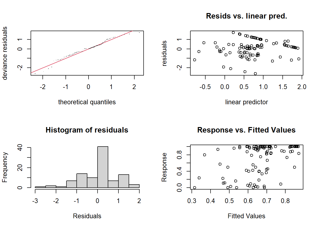
Method: ML   Optimizer: outer newton
full convergence after 10 iterations.
Gradient range [-5.252597e-05,-1.740295e-06]
(score -302.1485 & scale 1).
Hessian positive definite, eigenvalue range [1.740291e-06,67.0835].
Model rank =  46 / 46

Basis dimension (k) checking results. Low p-value (k-index<1) may
indicate that k is too low, especially if edf is close to k'.

                                           k'      edf k-index p-value
s(causalness_lagged)                 9.00e+00 1.00e+00    0.94    0.25
s(causalness_lagged):languageItalian 9.00e+00 6.16e-05    0.94    0.17
s(causalness_lagged):languageSpanish 9.00e+00 4.85e-05    0.94    0.26
s(causalness_degree):languageItalian 9.00e+00 1.40e+00    1.03    0.60
s(causalness_degree):languageSpanish 9.00e+00 4.98e-05    1.03    0.56
# --- 2. Concurvity (nonlinear collinearity among smooths) ---
concurvity(model5, full = TRUE) para s(causalness_lagged) s(causalness_lagged):languageItalian
worst 0.4633079 1.0000000 1.0000000
observed 0.4633079 1.0000000 1.0000000
estimate 0.4633079 0.9986535 0.9193622
s(causalness_lagged):languageSpanish
worst 1.0000000
observed 1.0000000
estimate 0.9536625
s(causalness_degree):languageItalian
worst 0.7057063
observed 0.5251884
estimate 0.2893153
s(causalness_degree):languageSpanish
worst 0.6903573
observed 0.5590216
estimate 0.3517013The QQ plot of residuals (gam.check) showed that the observed residuals closely followed the expected theoretical quantiles, with only minor deviations in the tails, suggesting that the beta regression model adequately captured the distributional assumptions.
The residuals–fitted plot showed that most observations clustered around mid-range fitted values (≈0.5), with residuals centered near zero and no clear systematic trends, indicating that the mean–variance structure of the beta GAM was generally appropriate. A descending line of points between fitted values of roughly 0–2, running from residuals > 1 down toward 0, suggests that a small subset of observations exhibits a systematic pattern, likely due to extreme fitted values, influential cases, or responses near the boundaries of the beta distribution. This pattern is localized rather than global, and the remainder of the residual cloud displays no indication of model misspecification.
The histogram of residuals indicates that most residuals are tightly clustered around zero, with only a small number of larger positive or negative residuals. Overall, the distribution appears approximately symmetric with light tails, suggesting no major problems with the residual structure or the appropriateness of the beta regression model.
Basis dimension checks (k-index = 0.94–1.03, all p > 0.2) indicated that the chosen number of knots (k = 10) was adequate, with no evidence of undersmoothing.
Concurvity checks indicated very high redundancy between the main smooth of causalness_lagged and its by-language interactions (concurvity ≈ 0.92–1.0). This suggests that the shared and language-specific smooths are not easily separable, likely because the language-specific effects were negligible. Concurvity among the causalness_degree smooths was low to moderate (≤ 0.56 observed), and therefore not considered problematic.
Visualise the results model5
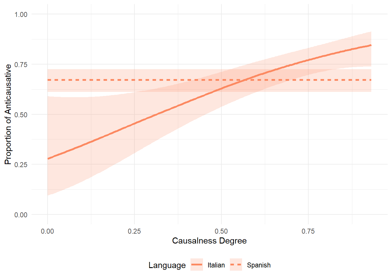
Visualisation of the effect of causalness_lagged, causalness_lagged by language and causalness_degree by language of model5 (now renamed model).
When plotting the group-wise interaction of causalness_lagged we see that Italian and Spanish essentially overlap. It is quite puzzling that the model selection suggested to keep it, as there is clearly no effect. We take it to mean that the real effect is the one of causalness_lagged by itself, it is capturing everything important. The group-specific smooths are essentially flat → not adding meaningful information. Statistically, the likelihood test picks up the tiniest difference, but for interpretation and visualization, it’s safe to consider them redundant.
model <- model5


# ---- 1. Prediction grid for causalness_lagged (shared smooth) ----
newdata_lagged <- tibble(
  causalness_lagged = seq(min(join$causalness_lagged), max(join$causalness_lagged), length.out = 200),
  causalness_degree = mean(join$causalness_degree, na.rm = TRUE),
  language = factor("Italian", levels = levels(join$language))  # shared smooth
)

pred_lagged <- predict(model, newdata_lagged, type = "link", se.fit = TRUE)

newdata_lagged <- newdata_lagged %>%
  mutate(
    fit_link  = pred_lagged$fit,
    se_link   = pred_lagged$se.fit,
    fit_resp  = plogis(fit_link),
    lower_resp = plogis(fit_link - 2 * se_link),
    upper_resp = plogis(fit_link + 2 * se_link)
  )

p_lagged <- ggplot(newdata_lagged, aes(x = causalness_lagged)) +
  geom_line(aes(y = fit_resp), color = "#fc8961", linewidth = 1.2) +
  geom_ribbon(aes(ymin = lower_resp, ymax = upper_resp), fill = "#fc8961", alpha = 0.2) +
  labs(x = "Causalness Lagged", y = "Proportion of Anticausative") +
  ylim(0, 1) +
  theme_minimal()

# ---- 2. Prediction grid for causalness_degree by language (interaction) ----
newdata_degree <- expand.grid(
  causalness_degree = seq(min(join$causalness_degree, na.rm = TRUE), max(join$causalness_degree, na.rm = TRUE), length.out = 200),
  language = levels(join$language)
) %>%
  as_tibble() %>%
  mutate(
    causalness_lagged = mean(join$causalness_lagged, na.rm = TRUE),
    language = factor(language, levels = levels(join$language))
  )

pred_degree <- predict(model, newdata_degree, type = "link", se.fit = TRUE)

newdata_degree <- newdata_degree %>%
  mutate(
    fit_link   = pred_degree$fit,
    se_link    = pred_degree$se.fit,
    fit_resp   = plogis(fit_link),
    lower_resp = plogis(fit_link - 2 * se_link),
    upper_resp = plogis(fit_link + 2 * se_link)
  )

p_degree_int <- ggplot(newdata_degree, aes(x = causalness_degree, y = fit_resp, linetype = language)) +
  geom_line(color = "#fc8961", linewidth = 1.2) +
  geom_ribbon(aes(ymin = lower_resp, ymax = upper_resp), fill = "#fc8961", alpha = 0.2, color = NA) +
  labs(x = "Causalness Degree", y = "Proportion of Anticausative", linetype = "Language") +
  ylim(0, 1) +
  theme_minimal() +
  theme(legend.position = "bottom")


# ---- 4. Prediction grid for causalness_lagged by language (interaction) ----
newdata_lagged_int <- expand.grid(
  causalness_lagged = seq(min(join$causalness_lagged), max(join$causalness_lagged), length.out = 200),
  language = levels(join$language)
) %>%
  as_tibble() %>%
  mutate(
    causalness_degree = mean(join$causalness_degree, na.rm = TRUE),
    language = factor(language, levels = levels(join$language))
  )

pred_lagged_int <- predict(model, newdata_lagged_int, type = "link", se.fit = TRUE)

newdata_lagged_int <- newdata_lagged_int %>%
  mutate(
    fit_link   = pred_lagged_int$fit,
    se_link    = pred_lagged_int$se.fit,
    fit_resp   = plogis(fit_link),
    lower_resp = plogis(fit_link - 2 * se_link),
    upper_resp = plogis(fit_link + 2 * se_link)
  )

p_lagged_int <- ggplot(newdata_lagged_int, aes(x = causalness_lagged, y = fit_resp, linetype = language)) +
  geom_line(color = "#fc8961", linewidth = 1.2) +
  geom_ribbon(aes(ymin = lower_resp, ymax = upper_resp), fill = "#fc8961", alpha = 0.2, color = NA) +
  labs(
    x = "Causalness Lagged",
    y = "Proportion of Anticausative",
    linetype = "Language"
  ) +
  ylim(0, 1) +
  theme_minimal() +
  theme(legend.position = "bottom")


p_lagged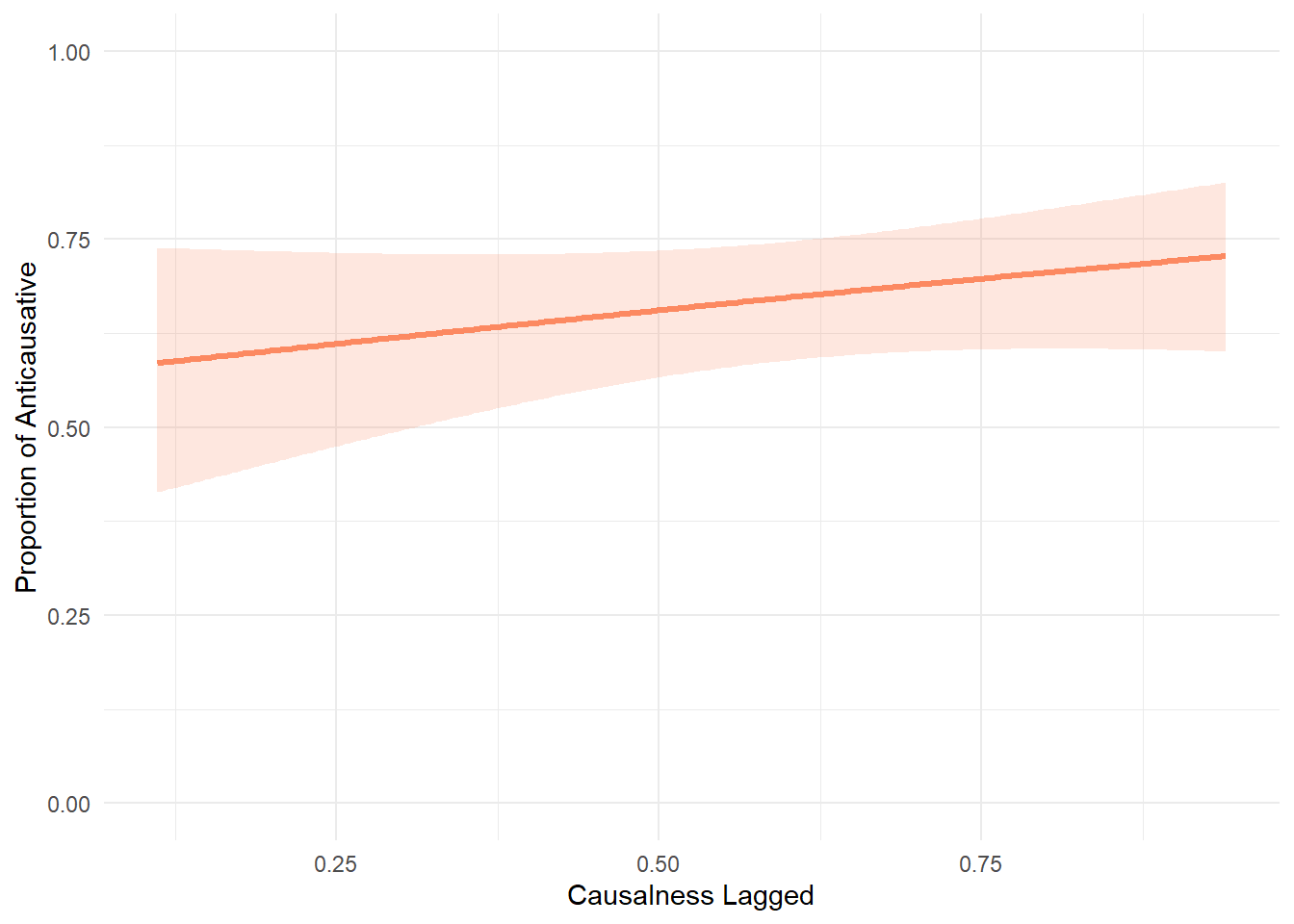
p_lagged_int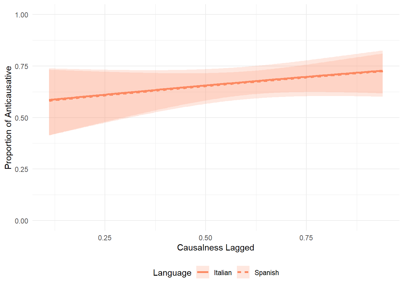
p_degree_int